Class Meeting 15 (1) Review of STAT 545
15.1 Today’s Agenda
- Part 1: Introductions and course overview (10 mins)
- Two parts to the course: reproducible workflows and dashboards
- Course grading elements
- Group projects
- Optional “lab”
- Office hours
- What to expect in STAT 547
- Part 2: Group projects in STAT 547 (10 mins)
- Partners
- Choosing a research question
- What’s due this week
- Part 3: Review of STAT545 (45 mins)
- tidy data
- ggplot
- dplyr
- File I/O
- Other stuff
15.2 Part 1: Introductions and course overview (15 mins)
STAT 547 can roughly be divided into two main ideas or themes: reproducible workflows and interactive dashboards. In the first part of the course we will start working with writing functions in R scripts and think a little bit about functional programming. Then with some new tools at our disposal, we will create “analysis pipelines” to automate and streamline the process going from loading raw data, all the way to creating a final report with the results of a regression analysis. Next we’ll switch gears and use our functional programming skills to create a dashboard app with multiple interactive components and multi-page/tab layouts. Finally we will end with deploying our dashboard to a free cloud service so that it is publicly available! It is my hope that you will use the things we learn in this course to inform your own data analysis pipelines in your PhD and Masters research projects. To that end, if you ever have questions about these tools could be used in your projects, feel free to drop by my office hours and I’d be happy to discuss it!
15.2.1 Important links
All course announcements, discussions, and participation worksheets will be posted: https://github.com/STAT547-UBC-2019-20/Discussions
The STAT 547 GitHub organization can be accessed here: https://github.com/STAT547-UBC-2019-20
All assignment/milestone/participation submissions are to be done on Canvas (submit URL of tagged release in your repo)
15.2.2 Course structure
(10%) Participation: Each week there will be two 90 minute classes closely following this guidebook. I hope to begin each meeting with a short introduction to provide some motivation for the topic of the day. We will then do coding exercises together. These will be due at the **end of the course* in your
participationrepository. Each file will be graded as complete (1), half-complete (0.5), or missing (0). Of the 12 class meetings, your 10 best will be used.(20%) Assignments: These will be short assignments designed to help you practice material from the current week. Your lowest assignment score will be dropped (so 5 of 6 assignments will count for your grade). Links to your
assignment_Xrepo should be submitted on Canvas and will be due on Saturdays at 6 PM.(60%) Team projects: There will be two team projects in this course (each equally weighted), one building an analysis pipeline and the second creating a dashboard using DashR. You will stay with the same groups for the duration of the course and both partners will receive the same grade. Though the projects are separate, they will use the same dataset and should be considered as extensions of each other. Links to your tagged release in your group project rep (
group_##_SOME_RELATED_NAME) repo should be submitted on Canvas and will be due on Saturdays at 6 PM.(10%) Teamwork: The teamwork document will be due after the end of each project and is your opportunity to reflect on your group dynamics and share with the teaching team your successess and challenges. It will constitute a 4 point rating scale on a few categories as well as an area for written feedback. A template teamwork document will be provided to you. This is not intended to be a long written exercise (unless you choose to do so, we will read it all).
I have added a 48-hour grace period for all submissions - this means that should “life happen”, you will still be able to submit your assignments for full credit up to 48 hours after the due date. You do not need to inform the teaching team if you need to use the grace period. After the 48 hour grace period, solutions will be released and no submissions will be accepted - no exceptions.
15.2.3 Office hours and optional “lab”
Each week there will be about 3 office hours scheduled. Check the course website for details on the office hour schedule.
15.2.4 Auditing students
You’re more than welcome to audit the course!
However, given the nature of this course, it will NOT mean any reduction in workload.
Auditing students will be:
- Graded on a Pass/Fail basis for each assignment/course activity
- Exempted from the peer review portion (assignment) of the course
- Doing the team project as an individual project (with no other change in scope or requirements)
If you would like to audit the course, you must submit the request by 11:59 PM on Thursday March 5th, 2020. After this - without exceptions - students will not be permitted to switch to (or from) audit status.
15.3 Part 2: Group projects in STAT 547
15.3.1 Partners
Your partners for the group projects will be randomly assigned using an algorithm with no human intervention. Teams will be posted on Canvas. There will be a “milestone” assignment due each week where you will be expected to work with your partner collaboratively in a single GitHub repository using the workflows you started learning about in STAT 545. The skills you learn in project courses working with git and GitHub will be essential for your future career - especially if it involves any amount of code.
15.3.2 Milestone 1
In the first milestone, your task is to introduce yourself to your project partner, exchange contact information, choose a dataset, and do some preliminary EDA on the dataset. We will talk about formulating a research question later on in the course, but keep in mind you will be doing a linear regression analysis to answer a particular research question. Keep in mind that you will be working with the dataset you choose for the remainder of the course, so I’ve provided some guidelines for choosing a dataset. Best of luck - this project course will be tonnes of fun !
15.4 Part 3: Review of STAT545 (45 mins)
15.5 Participation worksheet
- Download the participation worksheet from here
- Add it to your local clone of your participation repo (don’t forget to “accept” your participation repo first)
- Today’s participation activities are all at the end, in the section “Do I need more practice with the tidyverse?”
15.5.1 Introduction
This section is adapted from Chapter 3 of the tidynomicon textbook by Greg Wilson.
15.5.2 The Tidyverse
There is no point learning a language designed for data manipulation if you do not then bend data to your will. This chapter therefore looks at how to do the things that R was summoned—er, designed—to do.
15.5.3 Learning Objectives
- Install and load packages in R.
- Read CSV data with R.
- Explain what a tibble is and how tibbles related to data frames and matrices.
- Describe how
read_csvinfers data types for columns in tabular datasets. - Name and use three functions for inspects tibbles.
- Select subsets of tabular data using column names, scalar indices, ranges, and logical expressions.
- Explain the difference between indexing with
[and with[[. - Name and use four functions for calculating aggregate statistics on tabular data.
- Explain how these functions treat
NAby default, and how to change that behavior.
15.5.4 How do I read data?
We begin by looking at the file infant_hiv.csv, a tidied version of data on the percentage of infants born to women with HIV who received an HIV test themselves within two months of birth.
The original data comes from the UNICEF site at https://data.unicef.org/resources/dataset/hiv-aids-statistical-tables/,
and this file contains:
country,year,estimate,hi,lo
AFG,2009,NA,NA,NA
AFG,2010,NA,NA,NA
...
AFG,2017,NA,NA,NA
AGO,2009,NA,NA,NA
AGO,2010,0.03,0.04,0.02
AGO,2011,0.05,0.07,0.04
AGO,2012,0.06,0.08,0.05
...
ZWE,2016,0.71,0.88,0.62
ZWE,2017,0.65,0.81,0.57
The actual file has many more rows (and no ellipses).
It uses NA to show missing data rather than (for example) -, a space, or a blank,
and its values are interpreted as follows:
| Header | Datatype | Description |
|---|---|---|
| country | char | ISO3 country code of country reporting data |
| year | integer | year CE for which data reported |
| estimate | double/NA | estimated percentage of measurement |
| hi | double/NA | high end of range |
| lo | double/NA | low end of range |
We will import this data first by installing (if necessary, using install.packages("tidyverse")) the tidyverse collection of packages and then calling the read_csv function.
Loading the tidyverse gives us eight packages (ggplot2, tibble, tidyr, readr, purr, dplyr, stringr, forcats.
One of those, dplyr, defines two functions that mask standard functions in R with the same names.
If we need the originals, we can always get them with their fully-qualified names referring to the original package they belong to: stats::filter and stats::lag.
Firas’ note: I find these errors and messages quite irritating so I have made it so they do not appear unless I explicitly ask it to (which I did in this case for illustrative purposes).
At any time, we can call sessionInfo() to find out what versions of which packages we have loaded, along with the version of R we’re using and some other useful information:
## R version 3.6.2 (2017-01-27)
## Platform: x86_64-pc-linux-gnu (64-bit)
## Running under: Ubuntu 16.04.6 LTS
##
## Matrix products: default
## BLAS:   /home/travis/R-bin/lib/R/lib/libRblas.so
## LAPACK: /home/travis/R-bin/lib/R/lib/libRlapack.so
##
## locale:
##  [1] LC_CTYPE=en_US.UTF-8       LC_NUMERIC=C
##  [3] LC_TIME=en_US.UTF-8        LC_COLLATE=en_US.UTF-8
##  [5] LC_MONETARY=en_US.UTF-8    LC_MESSAGES=en_US.UTF-8
##  [7] LC_PAPER=en_US.UTF-8       LC_NAME=C
##  [9] LC_ADDRESS=C               LC_TELEPHONE=C
## [11] LC_MEASUREMENT=en_US.UTF-8 LC_IDENTIFICATION=C
##
## attached base packages:
## [1] stats     graphics  grDevices utils     datasets  methods   base
##
## other attached packages:
##  [1] readxl_1.3.1    DT_0.13         here_0.1        tsibble_0.8.6
##  [5] lubridate_1.7.4 scales_1.1.0    gapminder_0.3.0 forcats_0.5.0
##  [9] stringr_1.4.0   dplyr_0.8.5     purrr_0.3.3     readr_1.3.1
## [13] tidyr_1.0.2     tibble_3.0.0    ggplot2_3.3.0   tidyverse_1.3.0
##
## loaded via a namespace (and not attached):
##  [1] Rcpp_1.0.4        lattice_0.20-38   utf8_1.1.4        assertthat_0.2.1
##  [5] rprojroot_1.3-2   digest_0.6.25     plyr_1.8.6        R6_2.4.1
##  [9] cellranger_1.1.0  ggridges_0.5.2    backports_1.1.5   reprex_0.3.0
## [13] evaluate_0.14     highr_0.8         httr_1.4.1        pillar_1.4.3
## [17] rlang_0.4.5       rematch_1.0.1     curl_4.3          rstudioapi_0.11
## [21] rmarkdown_2.1     labeling_0.3      htmlwidgets_1.5.1 munsell_0.5.0
## [25] broom_0.5.5       anytime_0.3.7     compiler_3.6.2    modelr_0.1.6
## [29] xfun_0.12         pkgconfig_2.0.3   htmltools_0.4.0   tidyselect_1.0.0
## [33] bookdown_0.18     fansi_0.4.1       crayon_1.3.4      dbplyr_1.4.2
## [37] withr_2.1.2       grid_3.6.2        nlme_3.1-142      jsonlite_1.6.1
## [41] gtable_0.3.0      lifecycle_0.2.0   DBI_1.1.0         magrittr_1.5
## [45] cli_2.0.2         stringi_1.4.6     farver_2.0.3      fs_1.4.0
## [49] xml2_1.3.0        ellipsis_0.3.0    generics_0.0.2    vctrs_0.2.4
## [53] cowplot_1.0.0     tools_3.6.2       glue_1.3.2        crosstalk_1.1.0.1
## [57] hms_0.5.3         yaml_2.2.1        colorspace_1.4-1  rvest_0.3.5
## [61] knitr_1.28        haven_2.2.0
Once we have the tidyverse loaded, reading the file looks remarkably like reading the file:
R’s read_csv tells us a little about what it has done.
In particular, it guesses the data types of columns based on the first thousand values
and then tells us what types it has inferred.
(In a better universe, people would habitually use the first two rows of their spreadsheets for name and units, but we do not live there.)
We can now look at what read_csv has produced:
## # A tibble: 1,728 x 5
##    country  year estimate    hi    lo
##    <chr>   <dbl>    <dbl> <dbl> <dbl>
##  1 AFG      2009       NA    NA    NA
##  2 AFG      2010       NA    NA    NA
##  3 AFG      2011       NA    NA    NA
##  4 AFG      2012       NA    NA    NA
##  5 AFG      2013       NA    NA    NA
##  6 AFG      2014       NA    NA    NA
##  7 AFG      2015       NA    NA    NA
##  8 AFG      2016       NA    NA    NA
##  9 AFG      2017       NA    NA    NA
## 10 AGO      2009       NA    NA    NA
## # … with 1,718 more rows
This is a tibble, which is the tidyverse’s enhanced version of R’s data.frame.
It organizes data into named columns, each having one value for each row.
In statistical terms, the columns are the variables being observed and the rows are the actual observations.
15.5.5 How do I inspect data?
We often have a quick look at the content of a table to remind ourselves what it contains.
R has head and tail functions:
## # A tibble: 6 x 5
##   country  year estimate    hi    lo
##   <chr>   <dbl>    <dbl> <dbl> <dbl>
## 1 AFG      2009       NA    NA    NA
## 2 AFG      2010       NA    NA    NA
## 3 AFG      2011       NA    NA    NA
## 4 AFG      2012       NA    NA    NA
## 5 AFG      2013       NA    NA    NA
## 6 AFG 2014 NA NA NA## # A tibble: 6 x 5
## country year estimate hi lo
## <chr> <dbl> <dbl> <dbl> <dbl>
## 1 ZWE 2012 0.38 0.47 0.33
## 2 ZWE 2013 0.570 0.7 0.49
## 3 ZWE 2014 0.54 0.67 0.47
## 4 ZWE 2015 0.59 0.73 0.51
## 5 ZWE 2016 0.71 0.88 0.62
## 6 ZWE 2017 0.65 0.81 0.570Let’s have a closer look at that last command’s output:
## # A tibble: 6 x 5
##   country  year estimate    hi    lo
##   <chr>   <dbl>    <dbl> <dbl> <dbl>
## 1 ZWE      2012    0.38   0.47 0.33
## 2 ZWE      2013    0.570  0.7  0.49
## 3 ZWE      2014    0.54   0.67 0.47
## 4 ZWE      2015    0.59   0.73 0.51
## 5 ZWE      2016    0.71   0.88 0.62
## 6 ZWE 2017 0.65 0.81 0.570Note that the row numbers printed by tail are relative to the output, not absolute to the table.
What about overall information?
##    country               year         estimate           hi
##  Length:1728        Min.   :2009   Min.   :0.000   Min.   :0.0000
##  Class :character   1st Qu.:2011   1st Qu.:0.100   1st Qu.:0.1400
##  Mode  :character   Median :2013   Median :0.340   Median :0.4350
##                     Mean   :2013   Mean   :0.387   Mean   :0.4614
##                     3rd Qu.:2015   3rd Qu.:0.620   3rd Qu.:0.7625
##                     Max.   :2017   Max.   :0.950   Max.   :0.9500
##                                    NA's   :1000    NA's   :1000
##        lo
##  Min.   :0.0000
##  1st Qu.:0.0800
##  Median :0.2600
##  Mean   :0.3221
##  3rd Qu.:0.5100
##  Max.   :0.9500
##  NA's   :1000
Your display of R’s summary may or may not wrap, depending on how large a screen the older acolytes have allowed you.
15.5.6 How do I index rows and columns?
To access columns in R, you can use an attribute name:
## # A tibble: 1,728 x 1
##    estimate
##       <dbl>
##  1       NA
##  2       NA
##  3       NA
##  4       NA
##  5       NA
##  6       NA
##  7       NA
##  8       NA
##  9       NA
## 10       NA
## # … with 1,718 more rows
However, this syntax infant_hiv$estimate provides all the data:
##    [1]   NA   NA   NA   NA   NA   NA   NA   NA   NA   NA 0.03 0.05 0.06 0.15
##   [15] 0.10 0.06 0.01 0.01   NA   NA   NA   NA   NA   NA   NA   NA   NA   NA
##   [29]   NA   NA   NA   NA   NA   NA   NA   NA   NA   NA   NA   NA   NA   NA
##   [43]   NA   NA   NA   NA   NA 0.13 0.12 0.12 0.52 0.53 0.67 0.66   NA   NA
##   [57]   NA   NA   NA   NA   NA   NA   NA   NA   NA   NA   NA   NA   NA   NA
##   [71]   NA   NA   NA   NA   NA   NA   NA   NA   NA   NA   NA   NA   NA   NA
##   [85]   NA   NA   NA   NA   NA   NA 0.26 0.24 0.38 0.55 0.61 0.74 0.83 0.75
##   [99] 0.74   NA 0.10 0.10 0.11 0.18 0.12 0.02 0.12 0.20   NA   NA   NA   NA
##  [113]   NA   NA   NA   NA   NA   NA   NA 0.10 0.09 0.12 0.26 0.27 0.25 0.32
##  [127] 0.03 0.09 0.13 0.19 0.25 0.30 0.28 0.15 0.16   NA 0.02 0.02 0.02 0.03
##  [141] 0.15 0.10 0.17 0.14   NA   NA   NA   NA   NA   NA   NA   NA   NA   NA
##  [155]   NA   NA   NA   NA   NA   NA   NA   NA   NA   NA   NA   NA   NA   NA
##  [169]   NA   NA   NA   NA   NA   NA   NA   NA   NA   NA   NA   NA 0.95 0.95
##  [183] 0.95 0.95 0.95 0.95 0.80 0.95 0.87 0.77 0.75 0.72 0.51 0.55 0.50 0.62
##  [197] 0.37 0.36 0.07 0.46 0.46 0.46 0.46 0.44 0.43 0.42 0.40 0.25 0.25 0.46
##  [211] 0.25 0.45 0.45 0.46 0.46 0.45   NA   NA   NA   NA   NA   NA   NA   NA
##  [225]   NA   NA   NA   NA   NA   NA   NA   NA   NA   NA   NA   NA   NA   NA
##  [239]   NA   NA   NA   NA   NA   NA 0.53 0.35 0.36 0.48 0.41 0.45 0.47 0.50
##  [253] 0.01 0.01 0.07 0.05 0.03 0.09 0.12 0.21 0.23   NA   NA   NA   NA   NA
##  [267]   NA   NA   NA   NA   NA   NA   NA   NA   NA   NA   NA   NA   NA   NA
##  [281]   NA 0.64 0.56 0.67 0.77 0.92 0.70 0.85   NA   NA   NA   NA   NA   NA
##  [295]   NA   NA   NA   NA 0.22 0.03 0.19 0.12 0.33 0.28 0.39 0.40 0.27 0.20
##  [309] 0.25 0.30 0.32 0.36 0.33 0.53 0.51   NA 0.03 0.05 0.07 0.10 0.14 0.16
##  [323] 0.20 0.34 0.08 0.07 0.03 0.05 0.04 0.00 0.01 0.02 0.03   NA   NA   NA
##  [337]   NA   NA   NA   NA   NA   NA 0.05 0.10 0.18 0.22 0.30 0.37 0.45 0.44
##  [351] 0.48   NA   NA   NA   NA   NA   NA   NA   NA   NA 0.95 0.95 0.95 0.76
##  [365] 0.85 0.94 0.70 0.94 0.93 0.92 0.69 0.66 0.89 0.66 0.78 0.79 0.64 0.71
##  [379] 0.83 0.95 0.95 0.95 0.95 0.92 0.95 0.95 0.95   NA   NA   NA   NA   NA
##  [393]   NA   NA   NA   NA   NA   NA   NA   NA   NA   NA   NA   NA   NA   NA
##  [407]   NA   NA   NA   NA   NA   NA   NA   NA   NA   NA 0.02 0.08 0.08 0.02
##  [421] 0.08 0.10 0.10   NA   NA   NA   NA   NA   NA   NA   NA   NA   NA   NA
##  [435]   NA   NA   NA   NA   NA   NA   NA 0.28 0.10 0.43 0.46 0.64 0.95 0.95
##  [449] 0.72 0.80   NA   NA 0.38 0.23 0.55 0.27 0.23 0.33 0.61 0.01 0.01 0.95
##  [463] 0.87 0.21 0.87 0.54 0.70 0.69 0.04 0.05 0.04 0.04 0.04 0.05 0.07 0.10
##  [477] 0.11   NA   NA   NA   NA 0.27 0.39 0.36 0.39 0.15   NA   NA   NA   NA
##  [491]   NA   NA   NA   NA   NA   NA   NA   NA   NA   NA   NA   NA   NA   NA
##  [505] 0.04 0.40 0.15 0.24 0.24 0.25 0.31 0.45 0.38   NA   NA   NA   NA   NA
##  [519]   NA   NA   NA   NA   NA   NA   NA   NA   NA   NA   NA   NA   NA   NA
##  [533]   NA   NA   NA   NA   NA   NA   NA   NA   NA   NA   NA   NA   NA   NA
##  [547]   NA   NA   NA   NA 0.06 0.27 0.28 0.16 0.20 0.24 0.24 0.04   NA   NA
##  [561]   NA   NA   NA   NA   NA   NA   NA 0.61 0.82 0.69 0.62 0.58 0.74 0.77
##  [575] 0.79 0.84   NA 0.01 0.11 0.09 0.19 0.15 0.20 0.31 0.30   NA 0.05 0.06
##  [589] 0.00 0.06 0.07 0.04 0.39 0.11   NA   NA   NA   NA   NA 0.08 0.11 0.12
##  [603] 0.12   NA   NA 0.00 0.03 0.05 0.24 0.35 0.36 0.36   NA   NA   NA   NA
##  [617]   NA   NA   NA   NA   NA   NA   NA   NA   NA   NA   NA   NA   NA   NA
##  [631]   NA   NA   NA   NA   NA   NA   NA   NA   NA   NA   NA 0.19 0.17 0.11
##  [645] 0.15 0.15 0.15 0.17   NA 0.27 0.47 0.38 0.32 0.60 0.55 0.54 0.53 0.61
##  [659] 0.69 0.89 0.43 0.47 0.49 0.40 0.60 0.59   NA   NA   NA   NA   NA   NA
##  [673]   NA   NA   NA   NA   NA 0.04 0.39 0.35 0.36 0.32 0.35 0.40   NA   NA
##  [687]   NA   NA   NA   NA   NA   NA   NA   NA   NA   NA   NA 0.04 0.05 0.06
##  [701] 0.02 0.01   NA 0.06 0.07 0.08 0.09 0.10 0.25 0.27 0.23   NA   NA   NA
##  [715]   NA   NA   NA   NA   NA   NA 0.02 0.13 0.03 0.09 0.12 0.15 0.20 0.23
##  [729] 0.31   NA   NA   NA   NA   NA   NA   NA   NA   NA   NA   NA   NA   NA
##  [743]   NA   NA   NA   NA   NA   NA   NA   NA   NA   NA   NA   NA   NA   NA
##  [757]   NA   NA   NA   NA   NA   NA   NA   NA   NA   NA   NA 0.63   NA 0.68
##  [771] 0.59   NA   NA   NA   NA   NA   NA   NA   NA   NA   NA   NA   NA   NA
##  [785]   NA   NA   NA   NA   NA   NA   NA   NA 0.95 0.95 0.95 0.95 0.95 0.95
##  [799] 0.84 0.76 0.82   NA 0.75 0.46 0.45 0.45 0.74 0.51 0.56 0.51   NA   NA
##  [813] 0.03 0.11 0.11 0.38 0.33 0.66 0.70   NA 0.45 0.62 0.34 0.37 0.37 0.79
##  [827] 0.74 0.64   NA   NA   NA   NA   NA   NA   NA   NA   NA   NA   NA   NA
##  [841]   NA   NA   NA   NA   NA   NA   NA   NA   NA   NA   NA   NA   NA   NA
##  [855]   NA   NA 0.01 0.08 0.06 0.10 0.03 0.03 0.07 0.07   NA   NA   NA   NA
##  [869]   NA   NA   NA   NA   NA 0.05 0.05 0.17 0.28 0.31 0.13   NA   NA   NA
##  [883]   NA   NA   NA   NA   NA   NA   NA   NA   NA   NA   NA   NA   NA   NA
##  [897]   NA   NA   NA   NA   NA   NA   NA   NA   NA   NA   NA   NA   NA 0.43
##  [911] 0.95 0.95 0.70 0.47 0.51 0.87 0.58 0.51   NA   NA   NA   NA   NA   NA
##  [925]   NA   NA   NA   NA   NA   NA   NA   NA   NA   NA   NA   NA   NA   NA
##  [939]   NA   NA   NA   NA   NA   NA   NA 0.02 0.21 0.21 0.68 0.65 0.62 0.61
##  [953] 0.59 0.57 0.95 0.95 0.95 0.95 0.95 0.95 0.95 0.95 0.95   NA   NA 0.00
##  [967] 0.01   NA   NA   NA   NA   NA   NA   NA   NA   NA   NA   NA   NA   NA
##  [981]   NA   NA   NA   NA   NA   NA   NA   NA   NA   NA   NA   NA   NA   NA
##  [995]   NA   NA   NA   NA   NA   NA   NA   NA   NA   NA   NA   NA   NA   NA
## [1009] 0.08 0.08 0.08 0.10 0.08 0.06 0.03 0.11 0.11   NA   NA   NA   NA   NA
## [1023]   NA   NA   NA   NA   NA 0.01 0.04 0.05 0.09 0.12 0.15 0.26 0.28   NA
## [1037]   NA   NA   NA   NA   NA   NA   NA   NA   NA   NA   NA   NA   NA   NA
## [1051]   NA   NA   NA   NA 0.31 0.36 0.30 0.31 0.38 0.41 0.44 0.50   NA   NA
## [1065]   NA   NA   NA   NA   NA 0.08 0.08   NA   NA   NA   NA   NA   NA   NA
## [1079]   NA   NA   NA   NA   NA 0.06 0.17 0.21 0.20 0.31 0.52 0.37 0.61 0.68
## [1093] 0.68 0.77 0.87 0.75 0.69 0.95   NA 0.57 0.85 0.59 0.55 0.91 0.17 0.53
## [1107] 0.95   NA   NA   NA 0.01 0.09 0.02 0.11 0.05 0.10 0.04 0.06 0.07 0.06
## [1121] 0.05 0.06 0.10 0.11 0.12 0.50 0.38 0.95 0.47 0.57 0.51 0.65 0.60 0.75
## [1135]   NA   NA   NA   NA   NA   NA   NA   NA   NA   NA   NA   NA   NA   NA
## [1149]   NA   NA   NA   NA   NA   NA   NA   NA   NA   NA   NA   NA   NA 0.02
## [1163] 0.03 0.05 0.09 0.05 0.08 0.21 0.26 0.45   NA   NA   NA   NA   NA   NA
## [1177]   NA   NA   NA   NA   NA   NA   NA   NA   NA   NA   NA   NA   NA   NA
## [1191]   NA   NA   NA   NA   NA   NA   NA 0.01 0.01 0.01 0.00 0.01 0.01 0.00
## [1205] 0.00 0.01   NA 0.30 0.39 0.20 0.39 0.45 0.55 0.51 0.49   NA   NA 0.13
## [1219] 0.25 0.36 0.29 0.63 0.41 0.78 0.01 0.03 0.05 0.03 0.00 0.02 0.03 0.04
## [1233] 0.05   NA   NA   NA   NA   NA   NA   NA   NA   NA   NA   NA 0.23 0.18
## [1247] 0.53 0.30 0.37 0.36 0.35   NA   NA   NA   NA   NA   NA   NA   NA   NA
## [1261]   NA   NA   NA   NA   NA   NA   NA   NA   NA   NA   NA   NA   NA   NA
## [1275]   NA   NA   NA   NA   NA 0.27 0.34 0.50 0.39 0.38 0.47 0.52 0.52   NA
## [1289]   NA   NA   NA   NA   NA   NA   NA   NA   NA   NA   NA   NA   NA   NA
## [1303]   NA   NA   NA   NA   NA   NA   NA   NA 0.64 0.58 0.54 0.84 0.58 0.73
## [1317] 0.74 0.81 0.83 0.87 0.84 0.90 0.85   NA   NA   NA   NA   NA   NA   NA
## [1331]   NA   NA   NA   NA   NA   NA   NA   NA   NA   NA   NA 0.11 0.11 0.09
## [1345] 0.10 0.12 0.12 0.16 0.13 0.23   NA   NA   NA   NA   NA   NA   NA   NA
## [1359]   NA   NA   NA   NA   NA   NA   NA   NA   NA   NA   NA 0.01 0.01 0.02
## [1373] 0.25 0.02 0.03 0.06 0.07   NA 0.28 0.28 0.02 0.31 0.40 0.40 0.35 0.34
## [1387]   NA   NA   NA   NA   NA   NA   NA   NA   NA   NA   NA   NA   NA   NA
## [1401]   NA   NA   NA   NA   NA   NA   NA   NA   NA   NA 0.01 0.03 0.10   NA
## [1415]   NA   NA   NA   NA   NA   NA   NA   NA 0.09 0.09 0.09 0.34 0.58 0.81
## [1429] 0.95 0.95 0.67   NA   NA   NA   NA   NA   NA   NA   NA   NA   NA   NA
## [1443]   NA   NA   NA   NA   NA   NA   NA   NA   NA   NA   NA   NA   NA   NA
## [1457]   NA   NA   NA 0.50 0.93 0.95 0.87 0.84 0.88 0.82 0.81   NA   NA   NA
## [1471]   NA   NA   NA   NA   NA   NA   NA   NA   NA   NA   NA   NA   NA   NA
## [1485]   NA   NA 0.03 0.02 0.06 0.06 0.07 0.05 0.05 0.05 0.07 0.14 0.05 0.11
## [1499] 0.11 0.16 0.17 0.36 0.36   NA 0.54 0.56 0.64 0.68 0.70 0.92 0.92 0.94
## [1513] 0.01 0.04 0.08 0.11 0.14 0.14 0.30 0.21 0.43   NA   NA   NA   NA   NA
## [1527]   NA   NA   NA   NA   NA   NA   NA   NA   NA   NA   NA   NA   NA   NA
## [1541]   NA   NA   NA   NA   NA   NA   NA   NA   NA   NA   NA 0.37 0.50 0.95
## [1555] 0.83 0.90 0.94   NA   NA 0.16 0.14 0.18 0.33 0.40 0.31 0.13   NA   NA
## [1569]   NA   NA   NA   NA   NA   NA   NA   NA   NA   NA   NA   NA   NA   NA
## [1583]   NA   NA 0.13 0.24 0.30 0.29 0.29 0.39 0.38 0.39 0.36 0.08 0.13 0.38
## [1597] 0.45 0.50 0.69 0.43 0.35 0.48 0.78 0.95 0.81 0.88 0.95 0.78 0.47 0.55
## [1611] 0.48   NA   NA   NA   NA   NA   NA   NA   NA   NA   NA 0.62 0.68 0.85
## [1625] 0.95 0.95 0.95 0.90 0.95   NA   NA   NA   NA   NA   NA   NA   NA   NA
## [1639] 0.00 0.12 0.58 0.54 0.48 0.84 0.76 0.74 0.56   NA   NA   NA   NA   NA
## [1653]   NA   NA   NA   NA   NA   NA   NA   NA   NA   NA   NA   NA   NA   NA
## [1667]   NA 0.31 0.30 0.63 0.41 0.49 0.49 0.31   NA   NA   NA   NA   NA   NA
## [1681]   NA   NA   NA   NA   NA   NA   NA   NA   NA   NA   NA   NA   NA   NA
## [1695]   NA   NA   NA   NA   NA   NA   NA   NA 0.66 0.65 0.89 0.75 0.86 0.95
## [1709] 0.79 0.95 0.59 0.27 0.70 0.74 0.64 0.91 0.43 0.43 0.46   NA 0.12 0.23
## [1723] 0.38 0.57 0.54 0.59 0.71 0.65
Again, note that the boxed number on the left is the start index of that row.
What about single values? We have:
## [1] 0.05Ah—everything in R is a vector, so we get a vector of one value as an output rather than a single value.
## [1] 1And yes, ranges work:
## [1] NA NA NA NA NA 0.03 0.05 0.06 0.15 0.10Note that the upper bound inclusive in R. Note also that nothing prevents us from selecting a range of rows that spans several countries, which is why selecting by row number is usually a sign of innocence, insouciance, or desperation.
We can select by column number as well.
In R, a single index is interpreted as the column index:
## # A tibble: 1,728 x 1
##    country
##    <chr>
##  1 AFG
##  2 AFG
##  3 AFG
##  4 AFG
##  5 AFG
##  6 AFG
##  7 AFG
##  8 AFG
##  9 AFG
## 10 AGO
## # … with 1,718 more rows
But notice that the output is not a vector, but another tibble (i.e., a table with N rows and one column). This means that adding another index does column-wise indexing on that tibble:
## # A tibble: 1,728 x 1
##    country
##    <chr>
##  1 AFG
##  2 AFG
##  3 AFG
##  4 AFG
##  5 AFG
##  6 AFG
##  7 AFG
##  8 AFG
##  9 AFG
## 10 AGO
## # … with 1,718 more rows
How then are we to get the first mention of Afghanistan? The answer is to use double square brackets to strip away one level of structure:
##    [1] "AFG" "AFG" "AFG" "AFG" "AFG" "AFG" "AFG" "AFG" "AFG" "AGO" "AGO" "AGO"
##   [13] "AGO" "AGO" "AGO" "AGO" "AGO" "AGO" "AIA" "AIA" "AIA" "AIA" "AIA" "AIA"
##   [25] "AIA" "AIA" "AIA" "ALB" "ALB" "ALB" "ALB" "ALB" "ALB" "ALB" "ALB" "ALB"
##   [37] "ARE" "ARE" "ARE" "ARE" "ARE" "ARE" "ARE" "ARE" "ARE" "ARG" "ARG" "ARG"
##   [49] "ARG" "ARG" "ARG" "ARG" "ARG" "ARG" "ARM" "ARM" "ARM" "ARM" "ARM" "ARM"
##   [61] "ARM" "ARM" "ARM" "ATG" "ATG" "ATG" "ATG" "ATG" "ATG" "ATG" "ATG" "ATG"
##   [73] "AUS" "AUS" "AUS" "AUS" "AUS" "AUS" "AUS" "AUS" "AUS" "AUT" "AUT" "AUT"
##   [85] "AUT" "AUT" "AUT" "AUT" "AUT" "AUT" "AZE" "AZE" "AZE" "AZE" "AZE" "AZE"
##   [97] "AZE" "AZE" "AZE" "BDI" "BDI" "BDI" "BDI" "BDI" "BDI" "BDI" "BDI" "BDI"
##  [109] "BEL" "BEL" "BEL" "BEL" "BEL" "BEL" "BEL" "BEL" "BEL" "BEN" "BEN" "BEN"
##  [121] "BEN" "BEN" "BEN" "BEN" "BEN" "BEN" "BFA" "BFA" "BFA" "BFA" "BFA" "BFA"
##  [133] "BFA" "BFA" "BFA" "BGD" "BGD" "BGD" "BGD" "BGD" "BGD" "BGD" "BGD" "BGD"
##  [145] "BGR" "BGR" "BGR" "BGR" "BGR" "BGR" "BGR" "BGR" "BGR" "BHR" "BHR" "BHR"
##  [157] "BHR" "BHR" "BHR" "BHR" "BHR" "BHR" "BHS" "BHS" "BHS" "BHS" "BHS" "BHS"
##  [169] "BHS" "BHS" "BHS" "BIH" "BIH" "BIH" "BIH" "BIH" "BIH" "BIH" "BIH" "BIH"
##  [181] "BLR" "BLR" "BLR" "BLR" "BLR" "BLR" "BLR" "BLR" "BLR" "BLZ" "BLZ" "BLZ"
##  [193] "BLZ" "BLZ" "BLZ" "BLZ" "BLZ" "BLZ" "BOL" "BOL" "BOL" "BOL" "BOL" "BOL"
##  [205] "BOL" "BOL" "BOL" "BRA" "BRA" "BRA" "BRA" "BRA" "BRA" "BRA" "BRA" "BRA"
##  [217] "BRB" "BRB" "BRB" "BRB" "BRB" "BRB" "BRB" "BRB" "BRB" "BRN" "BRN" "BRN"
##  [229] "BRN" "BRN" "BRN" "BRN" "BRN" "BRN" "BTN" "BTN" "BTN" "BTN" "BTN" "BTN"
##  [241] "BTN" "BTN" "BTN" "BWA" "BWA" "BWA" "BWA" "BWA" "BWA" "BWA" "BWA" "BWA"
##  [253] "CAF" "CAF" "CAF" "CAF" "CAF" "CAF" "CAF" "CAF" "CAF" "CAN" "CAN" "CAN"
##  [265] "CAN" "CAN" "CAN" "CAN" "CAN" "CAN" "CHE" "CHE" "CHE" "CHE" "CHE" "CHE"
##  [277] "CHE" "CHE" "CHE" "CHL" "CHL" "CHL" "CHL" "CHL" "CHL" "CHL" "CHL" "CHL"
##  [289] "CHN" "CHN" "CHN" "CHN" "CHN" "CHN" "CHN" "CHN" "CHN" "CIV" "CIV" "CIV"
##  [301] "CIV" "CIV" "CIV" "CIV" "CIV" "CIV" "CMR" "CMR" "CMR" "CMR" "CMR" "CMR"
##  [313] "CMR" "CMR" "CMR" "COD" "COD" "COD" "COD" "COD" "COD" "COD" "COD" "COD"
##  [325] "COG" "COG" "COG" "COG" "COG" "COG" "COG" "COG" "COG" "COK" "COK" "COK"
##  [337] "COK" "COK" "COK" "COK" "COK" "COK" "COL" "COL" "COL" "COL" "COL" "COL"
##  [349] "COL" "COL" "COL" "COM" "COM" "COM" "COM" "COM" "COM" "COM" "COM" "COM"
##  [361] "CPV" "CPV" "CPV" "CPV" "CPV" "CPV" "CPV" "CPV" "CPV" "CRI" "CRI" "CRI"
##  [373] "CRI" "CRI" "CRI" "CRI" "CRI" "CRI" "CUB" "CUB" "CUB" "CUB" "CUB" "CUB"
##  [385] "CUB" "CUB" "CUB" "CYP" "CYP" "CYP" "CYP" "CYP" "CYP" "CYP" "CYP" "CYP"
##  [397] "CZE" "CZE" "CZE" "CZE" "CZE" "CZE" "CZE" "CZE" "CZE" "DEU" "DEU" "DEU"
##  [409] "DEU" "DEU" "DEU" "DEU" "DEU" "DEU" "DJI" "DJI" "DJI" "DJI" "DJI" "DJI"
##  [421] "DJI" "DJI" "DJI" "DMA" "DMA" "DMA" "DMA" "DMA" "DMA" "DMA" "DMA" "DMA"
##  [433] "DNK" "DNK" "DNK" "DNK" "DNK" "DNK" "DNK" "DNK" "DNK" "DOM" "DOM" "DOM"
##  [445] "DOM" "DOM" "DOM" "DOM" "DOM" "DOM" "DZA" "DZA" "DZA" "DZA" "DZA" "DZA"
##  [457] "DZA" "DZA" "DZA" "ECU" "ECU" "ECU" "ECU" "ECU" "ECU" "ECU" "ECU" "ECU"
##  [469] "EGY" "EGY" "EGY" "EGY" "EGY" "EGY" "EGY" "EGY" "EGY" "ERI" "ERI" "ERI"
##  [481] "ERI" "ERI" "ERI" "ERI" "ERI" "ERI" "ESP" "ESP" "ESP" "ESP" "ESP" "ESP"
##  [493] "ESP" "ESP" "ESP" "EST" "EST" "EST" "EST" "EST" "EST" "EST" "EST" "EST"
##  [505] "ETH" "ETH" "ETH" "ETH" "ETH" "ETH" "ETH" "ETH" "ETH" "FIN" "FIN" "FIN"
##  [517] "FIN" "FIN" "FIN" "FIN" "FIN" "FIN" "FJI" "FJI" "FJI" "FJI" "FJI" "FJI"
##  [529] "FJI" "FJI" "FJI" "FRA" "FRA" "FRA" "FRA" "FRA" "FRA" "FRA" "FRA" "FRA"
##  [541] "FSM" "FSM" "FSM" "FSM" "FSM" "FSM" "FSM" "FSM" "FSM" "GAB" "GAB" "GAB"
##  [553] "GAB" "GAB" "GAB" "GAB" "GAB" "GAB" "GBR" "GBR" "GBR" "GBR" "GBR" "GBR"
##  [565] "GBR" "GBR" "GBR" "GEO" "GEO" "GEO" "GEO" "GEO" "GEO" "GEO" "GEO" "GEO"
##  [577] "GHA" "GHA" "GHA" "GHA" "GHA" "GHA" "GHA" "GHA" "GHA" "GIN" "GIN" "GIN"
##  [589] "GIN" "GIN" "GIN" "GIN" "GIN" "GIN" "GMB" "GMB" "GMB" "GMB" "GMB" "GMB"
##  [601] "GMB" "GMB" "GMB" "GNB" "GNB" "GNB" "GNB" "GNB" "GNB" "GNB" "GNB" "GNB"
##  [613] "GNQ" "GNQ" "GNQ" "GNQ" "GNQ" "GNQ" "GNQ" "GNQ" "GNQ" "GRC" "GRC" "GRC"
##  [625] "GRC" "GRC" "GRC" "GRC" "GRC" "GRC" "GRD" "GRD" "GRD" "GRD" "GRD" "GRD"
##  [637] "GRD" "GRD" "GRD" "GTM" "GTM" "GTM" "GTM" "GTM" "GTM" "GTM" "GTM" "GTM"
##  [649] "GUY" "GUY" "GUY" "GUY" "GUY" "GUY" "GUY" "GUY" "GUY" "HND" "HND" "HND"
##  [661] "HND" "HND" "HND" "HND" "HND" "HND" "HRV" "HRV" "HRV" "HRV" "HRV" "HRV"
##  [673] "HRV" "HRV" "HRV" "HTI" "HTI" "HTI" "HTI" "HTI" "HTI" "HTI" "HTI" "HTI"
##  [685] "HUN" "HUN" "HUN" "HUN" "HUN" "HUN" "HUN" "HUN" "HUN" "IDN" "IDN" "IDN"
##  [697] "IDN" "IDN" "IDN" "IDN" "IDN" "IDN" "IND" "IND" "IND" "IND" "IND" "IND"
##  [709] "IND" "IND" "IND" "IRL" "IRL" "IRL" "IRL" "IRL" "IRL" "IRL" "IRL" "IRL"
##  [721] "IRN" "IRN" "IRN" "IRN" "IRN" "IRN" "IRN" "IRN" "IRN" "IRQ" "IRQ" "IRQ"
##  [733] "IRQ" "IRQ" "IRQ" "IRQ" "IRQ" "IRQ" "ISL" "ISL" "ISL" "ISL" "ISL" "ISL"
##  [745] "ISL" "ISL" "ISL" "ISR" "ISR" "ISR" "ISR" "ISR" "ISR" "ISR" "ISR" "ISR"
##  [757] "ITA" "ITA" "ITA" "ITA" "ITA" "ITA" "ITA" "ITA" "ITA" "JAM" "JAM" "JAM"
##  [769] "JAM" "JAM" "JAM" "JAM" "JAM" "JAM" "JOR" "JOR" "JOR" "JOR" "JOR" "JOR"
##  [781] "JOR" "JOR" "JOR" "JPN" "JPN" "JPN" "JPN" "JPN" "JPN" "JPN" "JPN" "JPN"
##  [793] "KAZ" "KAZ" "KAZ" "KAZ" "KAZ" "KAZ" "KAZ" "KAZ" "KAZ" "KEN" "KEN" "KEN"
##  [805] "KEN" "KEN" "KEN" "KEN" "KEN" "KEN" "KGZ" "KGZ" "KGZ" "KGZ" "KGZ" "KGZ"
##  [817] "KGZ" "KGZ" "KGZ" "KHM" "KHM" "KHM" "KHM" "KHM" "KHM" "KHM" "KHM" "KHM"
##  [829] "KIR" "KIR" "KIR" "KIR" "KIR" "KIR" "KIR" "KIR" "KIR" "KNA" "KNA" "KNA"
##  [841] "KNA" "KNA" "KNA" "KNA" "KNA" "KNA" "KOR" "KOR" "KOR" "KOR" "KOR" "KOR"
##  [853] "KOR" "KOR" "KOR" "LAO" "LAO" "LAO" "LAO" "LAO" "LAO" "LAO" "LAO" "LAO"
##  [865] "LBN" "LBN" "LBN" "LBN" "LBN" "LBN" "LBN" "LBN" "LBN" "LBR" "LBR" "LBR"
##  [877] "LBR" "LBR" "LBR" "LBR" "LBR" "LBR" "LBY" "LBY" "LBY" "LBY" "LBY" "LBY"
##  [889] "LBY" "LBY" "LBY" "LCA" "LCA" "LCA" "LCA" "LCA" "LCA" "LCA" "LCA" "LCA"
##  [901] "LKA" "LKA" "LKA" "LKA" "LKA" "LKA" "LKA" "LKA" "LKA" "LSO" "LSO" "LSO"
##  [913] "LSO" "LSO" "LSO" "LSO" "LSO" "LSO" "LTU" "LTU" "LTU" "LTU" "LTU" "LTU"
##  [925] "LTU" "LTU" "LTU" "LUX" "LUX" "LUX" "LUX" "LUX" "LUX" "LUX" "LUX" "LUX"
##  [937] "LVA" "LVA" "LVA" "LVA" "LVA" "LVA" "LVA" "LVA" "LVA" "MAR" "MAR" "MAR"
##  [949] "MAR" "MAR" "MAR" "MAR" "MAR" "MAR" "MDA" "MDA" "MDA" "MDA" "MDA" "MDA"
##  [961] "MDA" "MDA" "MDA" "MDG" "MDG" "MDG" "MDG" "MDG" "MDG" "MDG" "MDG" "MDG"
##  [973] "MDV" "MDV" "MDV" "MDV" "MDV" "MDV" "MDV" "MDV" "MDV" "MEX" "MEX" "MEX"
##  [985] "MEX" "MEX" "MEX" "MEX" "MEX" "MEX" "MHL" "MHL" "MHL" "MHL" "MHL" "MHL"
##  [997] "MHL" "MHL" "MHL" "MKD" "MKD" "MKD" "MKD" "MKD" "MKD" "MKD" "MKD" "MKD"
## [1009] "MLI" "MLI" "MLI" "MLI" "MLI" "MLI" "MLI" "MLI" "MLI" "MLT" "MLT" "MLT"
## [1021] "MLT" "MLT" "MLT" "MLT" "MLT" "MLT" "MMR" "MMR" "MMR" "MMR" "MMR" "MMR"
## [1033] "MMR" "MMR" "MMR" "MNE" "MNE" "MNE" "MNE" "MNE" "MNE" "MNE" "MNE" "MNE"
## [1045] "MNG" "MNG" "MNG" "MNG" "MNG" "MNG" "MNG" "MNG" "MNG" "MOZ" "MOZ" "MOZ"
## [1057] "MOZ" "MOZ" "MOZ" "MOZ" "MOZ" "MOZ" "MRT" "MRT" "MRT" "MRT" "MRT" "MRT"
## [1069] "MRT" "MRT" "MRT" "MUS" "MUS" "MUS" "MUS" "MUS" "MUS" "MUS" "MUS" "MUS"
## [1081] "MWI" "MWI" "MWI" "MWI" "MWI" "MWI" "MWI" "MWI" "MWI" "MYS" "MYS" "MYS"
## [1093] "MYS" "MYS" "MYS" "MYS" "MYS" "MYS" "NAM" "NAM" "NAM" "NAM" "NAM" "NAM"
## [1105] "NAM" "NAM" "NAM" "NER" "NER" "NER" "NER" "NER" "NER" "NER" "NER" "NER"
## [1117] "NGA" "NGA" "NGA" "NGA" "NGA" "NGA" "NGA" "NGA" "NGA" "NIC" "NIC" "NIC"
## [1129] "NIC" "NIC" "NIC" "NIC" "NIC" "NIC" "NIU" "NIU" "NIU" "NIU" "NIU" "NIU"
## [1141] "NIU" "NIU" "NIU" "NLD" "NLD" "NLD" "NLD" "NLD" "NLD" "NLD" "NLD" "NLD"
## [1153] "NOR" "NOR" "NOR" "NOR" "NOR" "NOR" "NOR" "NOR" "NOR" "NPL" "NPL" "NPL"
## [1165] "NPL" "NPL" "NPL" "NPL" "NPL" "NPL" "NRU" "NRU" "NRU" "NRU" "NRU" "NRU"
## [1177] "NRU" "NRU" "NRU" "NZL" "NZL" "NZL" "NZL" "NZL" "NZL" "NZL" "NZL" "NZL"
## [1189] "OMN" "OMN" "OMN" "OMN" "OMN" "OMN" "OMN" "OMN" "OMN" "PAK" "PAK" "PAK"
## [1201] "PAK" "PAK" "PAK" "PAK" "PAK" "PAK" "PAN" "PAN" "PAN" "PAN" "PAN" "PAN"
## [1213] "PAN" "PAN" "PAN" "PER" "PER" "PER" "PER" "PER" "PER" "PER" "PER" "PER"
## [1225] "PHL" "PHL" "PHL" "PHL" "PHL" "PHL" "PHL" "PHL" "PHL" "PLW" "PLW" "PLW"
## [1237] "PLW" "PLW" "PLW" "PLW" "PLW" "PLW" "PNG" "PNG" "PNG" "PNG" "PNG" "PNG"
## [1249] "PNG" "PNG" "PNG" "POL" "POL" "POL" "POL" "POL" "POL" "POL" "POL" "POL"
## [1261] "PRK" "PRK" "PRK" "PRK" "PRK" "PRK" "PRK" "PRK" "PRK" "PRT" "PRT" "PRT"
## [1273] "PRT" "PRT" "PRT" "PRT" "PRT" "PRT" "PRY" "PRY" "PRY" "PRY" "PRY" "PRY"
## [1285] "PRY" "PRY" "PRY" "PSE" "PSE" "PSE" "PSE" "PSE" "PSE" "PSE" "PSE" "PSE"
## [1297] "ROU" "ROU" "ROU" "ROU" "ROU" "ROU" "ROU" "ROU" "ROU" "RUS" "RUS" "RUS"
## [1309] "RUS" "RUS" "RUS" "RUS" "RUS" "RUS" "RWA" "RWA" "RWA" "RWA" "RWA" "RWA"
## [1321] "RWA" "RWA" "RWA" "SAU" "SAU" "SAU" "SAU" "SAU" "SAU" "SAU" "SAU" "SAU"
## [1333] "SDN" "SDN" "SDN" "SDN" "SDN" "SDN" "SDN" "SDN" "SDN" "SEN" "SEN" "SEN"
## [1345] "SEN" "SEN" "SEN" "SEN" "SEN" "SEN" "SGP" "SGP" "SGP" "SGP" "SGP" "SGP"
## [1357] "SGP" "SGP" "SGP" "SLB" "SLB" "SLB" "SLB" "SLB" "SLB" "SLB" "SLB" "SLB"
## [1369] "SLE" "SLE" "SLE" "SLE" "SLE" "SLE" "SLE" "SLE" "SLE" "SLV" "SLV" "SLV"
## [1381] "SLV" "SLV" "SLV" "SLV" "SLV" "SLV" "SOM" "SOM" "SOM" "SOM" "SOM" "SOM"
## [1393] "SOM" "SOM" "SOM" "SRB" "SRB" "SRB" "SRB" "SRB" "SRB" "SRB" "SRB" "SRB"
## [1405] "SSD" "SSD" "SSD" "SSD" "SSD" "SSD" "SSD" "SSD" "SSD" "STP" "STP" "STP"
## [1417] "STP" "STP" "STP" "STP" "STP" "STP" "SUR" "SUR" "SUR" "SUR" "SUR" "SUR"
## [1429] "SUR" "SUR" "SUR" "SVK" "SVK" "SVK" "SVK" "SVK" "SVK" "SVK" "SVK" "SVK"
## [1441] "SVN" "SVN" "SVN" "SVN" "SVN" "SVN" "SVN" "SVN" "SVN" "SWE" "SWE" "SWE"
## [1453] "SWE" "SWE" "SWE" "SWE" "SWE" "SWE" "SWZ" "SWZ" "SWZ" "SWZ" "SWZ" "SWZ"
## [1465] "SWZ" "SWZ" "SWZ" "SYC" "SYC" "SYC" "SYC" "SYC" "SYC" "SYC" "SYC" "SYC"
## [1477] "SYR" "SYR" "SYR" "SYR" "SYR" "SYR" "SYR" "SYR" "SYR" "TCD" "TCD" "TCD"
## [1489] "TCD" "TCD" "TCD" "TCD" "TCD" "TCD" "TGO" "TGO" "TGO" "TGO" "TGO" "TGO"
## [1501] "TGO" "TGO" "TGO" "THA" "THA" "THA" "THA" "THA" "THA" "THA" "THA" "THA"
## [1513] "TJK" "TJK" "TJK" "TJK" "TJK" "TJK" "TJK" "TJK" "TJK" "TKM" "TKM" "TKM"
## [1525] "TKM" "TKM" "TKM" "TKM" "TKM" "TKM" "TLS" "TLS" "TLS" "TLS" "TLS" "TLS"
## [1537] "TLS" "TLS" "TLS" "TON" "TON" "TON" "TON" "TON" "TON" "TON" "TON" "TON"
## [1549] "TTO" "TTO" "TTO" "TTO" "TTO" "TTO" "TTO" "TTO" "TTO" "TUN" "TUN" "TUN"
## [1561] "TUN" "TUN" "TUN" "TUN" "TUN" "TUN" "TUR" "TUR" "TUR" "TUR" "TUR" "TUR"
## [1573] "TUR" "TUR" "TUR" "TUV" "TUV" "TUV" "TUV" "TUV" "TUV" "TUV" "TUV" "TUV"
## [1585] "TZA" "TZA" "TZA" "TZA" "TZA" "TZA" "TZA" "TZA" "TZA" "UGA" "UGA" "UGA"
## [1597] "UGA" "UGA" "UGA" "UGA" "UGA" "UGA" "UKR" "UKR" "UKR" "UKR" "UKR" "UKR"
## [1609] "UKR" "UKR" "UKR" "UNK" "UNK" "UNK" "UNK" "UNK" "UNK" "UNK" "UNK" "UNK"
## [1621] "URY" "URY" "URY" "URY" "URY" "URY" "URY" "URY" "URY" "USA" "USA" "USA"
## [1633] "USA" "USA" "USA" "USA" "USA" "USA" "UZB" "UZB" "UZB" "UZB" "UZB" "UZB"
## [1645] "UZB" "UZB" "UZB" "VCT" "VCT" "VCT" "VCT" "VCT" "VCT" "VCT" "VCT" "VCT"
## [1657] "VEN" "VEN" "VEN" "VEN" "VEN" "VEN" "VEN" "VEN" "VEN" "VNM" "VNM" "VNM"
## [1669] "VNM" "VNM" "VNM" "VNM" "VNM" "VNM" "VUT" "VUT" "VUT" "VUT" "VUT" "VUT"
## [1681] "VUT" "VUT" "VUT" "WSM" "WSM" "WSM" "WSM" "WSM" "WSM" "WSM" "WSM" "WSM"
## [1693] "YEM" "YEM" "YEM" "YEM" "YEM" "YEM" "YEM" "YEM" "YEM" "ZAF" "ZAF" "ZAF"
## [1705] "ZAF" "ZAF" "ZAF" "ZAF" "ZAF" "ZAF" "ZMB" "ZMB" "ZMB" "ZMB" "ZMB" "ZMB"
## [1717] "ZMB" "ZMB" "ZMB" "ZWE" "ZWE" "ZWE" "ZWE" "ZWE" "ZWE" "ZWE" "ZWE" "ZWE"
This is now a plain old vector, so it can be indexed with single square brackets:
## [1] "AFG"But that too is a vector, so it can of course be indexed as well (for some value of “of course”):
## [1] "AFG"Thus, data[1][[1]] produces a tibble, then selects the first column vector from it, so it still gives us a vector.
This is not madness.
It is merely…differently sane.
Subsetting Data Frames
When we are working with data frames (including tibbles), subsetting with a single vector selects columns, not rows, because data frames are stored as lists of columns. This means that
df[1:2]selects two columns fromdf. However, indf[2:3, 1:2], the first index selects rows, while the second selects columns.
15.5.7 How do I calculate basic statistics?
What is the average estimate? We start by grabbing that column for convenience:
## [1] 1728## [1] NAThe void is always there, waiting for us…
Let’s fix this in R first by telling mean to drop NAs:
## [1] 0.3870192Many functions in R use na.rm to control whether NAs are removed or not.
(Remember, the . character is just another part of the name)
R’s default behavior is to leave NAs in, and then to include them in aggregate computations.
A good use of aggregation is to check the quality of the data. For example, we can ask if there are any records where some of the estimate, the low value, or the high value are missing,
## [1] FALSEAside: In R, there’s a handy package called glue.
The glue package is very useful for “gluing” strings to data in R.
Let’s load it to see how it works:
## min 0## max 0.95## sd 0.30345110742141115.5.8 How do I filter data?
By “filtering”, we mean “selecting records by value”.
The simplest approach is to use a vector of logical values to keep only the values corresponding to TRUE:
## [1] 1052## [1] NA NA NA NA NA NA NA NA NA NA NA NA NA NA
## [15] NA NA NA NA NA NA NA NA NA NA NA NA NA NA
## [29] NA NA NA NA NA NA NA NA NA NA NA NA NA NA
## [43] NA NA NA NA NA NA NA NA NA NA NA NA NA NA
## [57] NA NA NA NA NA NA NA NA NA NA NA NA NA NA
## [71] NA NA NA NA NA NA NA NA NA NA NA NA NA NA
## [85] NA NA NA NA NA NA NA NA NA NA NA NA NA NA
## [99] NA NA NA NA NA NA NA NA NA NA NA NA NA NA
## [113] NA NA NA NA NA NA NA NA NA NA NA NA 0.95 0.95
## [127] 0.95 0.95 0.95 0.95 0.95 NA NA NA NA NA NA NA NA NA
## [141] NA NA NA NA NA NA NA NA NA NA NA NA NA NA
## [155] NA NA NA NA NA NA NA NA NA NA NA NA NA NA
## [169] NA NA NA NA NA NA NA NA NA NA NA NA NA NA
## [183] NA NA NA NA NA NA NA NA NA NA NA NA NA NA
## [197] NA NA NA NA NA NA NA NA NA NA NA NA 0.95 0.95
## [211] 0.95 0.95 0.95 0.95 0.95 0.95 0.95 0.95 NA NA NA NA NA NA
## [225] NA NA NA NA NA NA NA NA NA NA NA NA NA NA
## [239] NA NA NA NA NA NA NA NA NA NA NA NA NA NA
## [253] NA NA NA NA NA NA NA NA NA NA NA NA NA 0.95
## [267] 0.95 NA NA 0.95 NA NA NA NA NA NA NA NA NA NA
## [281] NA NA NA NA NA NA NA NA NA NA NA NA NA NA
## [295] NA NA NA NA NA NA NA NA NA NA NA NA NA NA
## [309] NA NA NA NA NA NA NA NA NA NA NA NA NA NA
## [323] NA NA NA NA NA NA NA NA NA NA NA NA NA NA
## [337] NA NA NA NA NA NA NA NA NA NA NA NA NA NA
## [351] NA NA NA NA NA NA NA NA NA NA NA NA NA NA
## [365] NA NA NA NA NA NA NA NA NA NA NA NA NA NA
## [379] NA NA NA NA NA NA NA NA NA NA NA NA NA NA
## [393] NA NA NA NA NA NA NA NA NA NA NA NA NA NA
## [407] NA NA NA NA NA NA NA NA NA NA NA NA NA NA
## [421] NA NA NA NA NA NA NA NA NA NA NA NA NA NA
## [435] NA NA NA NA NA NA NA NA NA NA NA NA NA NA
## [449] NA NA NA NA NA NA NA NA NA NA NA NA NA NA
## [463] NA NA NA NA NA NA NA NA NA 0.95 0.95 0.95 0.95 0.95
## [477] 0.95 NA NA NA NA NA NA NA NA NA NA NA NA NA
## [491] NA NA NA NA NA NA NA NA NA NA NA NA NA NA
## [505] NA NA NA NA NA NA NA NA NA NA NA NA NA NA
## [519] NA NA NA NA NA NA NA NA NA NA NA NA NA NA
## [533] NA NA NA NA NA NA NA NA NA NA NA NA NA NA
## [547] NA NA 0.95 0.95 NA NA NA NA NA NA NA NA NA NA
## [561] NA NA NA NA NA NA NA NA NA NA NA NA NA NA
## [575] NA NA NA 0.95 0.95 0.95 0.95 0.95 0.95 0.95 0.95 0.95 NA NA
## [589] NA NA NA NA NA NA NA NA NA NA NA NA NA NA
## [603] NA NA NA NA NA NA NA NA NA NA NA NA NA NA
## [617] NA NA NA NA NA NA NA NA NA NA NA NA NA NA
## [631] NA NA NA NA NA NA NA NA NA NA NA NA NA NA
## [645] NA NA NA NA NA NA NA NA NA NA NA NA NA NA
## [659] NA NA NA NA NA NA NA NA NA NA NA NA NA NA
## [673] NA NA NA NA NA 0.95 NA 0.95 NA NA NA 0.95 NA NA
## [687] NA NA NA NA NA NA NA NA NA NA NA NA NA NA
## [701] NA NA NA NA NA NA NA NA NA NA NA NA NA NA
## [715] NA NA NA NA NA NA NA NA NA NA NA NA NA NA
## [729] NA NA NA NA NA NA NA NA NA NA NA NA NA NA
## [743] NA NA NA NA NA NA NA NA NA NA NA NA NA NA
## [757] NA NA NA NA NA NA NA NA NA NA NA NA NA NA
## [771] NA NA NA NA NA NA NA NA NA NA NA NA NA NA
## [785] NA NA NA NA NA NA NA NA NA NA NA NA NA NA
## [799] NA NA NA NA NA NA NA NA NA NA NA NA NA NA
## [813] NA NA NA NA NA NA NA NA NA NA NA NA NA NA
## [827] NA NA NA NA NA NA NA NA NA NA NA NA NA NA
## [841] NA NA NA NA NA NA NA NA NA NA NA NA NA NA
## [855] NA NA NA NA NA NA NA NA NA NA NA NA NA NA
## [869] NA NA NA NA NA NA 0.95 0.95 NA NA NA NA NA NA
## [883] NA NA NA NA NA NA NA NA NA NA NA NA NA NA
## [897] NA NA NA NA NA NA NA NA 0.95 NA NA NA NA NA
## [911] NA NA NA NA NA NA NA NA NA NA NA NA NA NA
## [925] NA NA NA NA NA NA NA NA NA NA NA NA NA NA
## [939] NA NA NA NA NA NA NA NA NA NA NA NA NA NA
## [953] NA NA NA 0.95 NA NA NA NA NA NA NA NA NA NA
## [967] NA NA NA NA NA NA NA NA NA NA 0.95 0.95 NA NA
## [981] NA NA NA NA NA NA NA NA 0.95 0.95 0.95 0.95 NA NA
## [995] NA NA NA NA NA NA NA NA NA NA NA NA NA NA
## [1009] NA NA NA NA NA NA NA NA NA NA NA NA NA NA
## [1023] NA NA NA NA NA NA NA NA NA NA NA NA NA NA
## [1037] NA NA NA NA NA NA NA NA NA NA NA NA NA 0.95
## [1051] 0.95 NAIt appears that R has kept the unknown values in order to highlight just how little we know.
More precisely, wherever there was an NA in the original data, there is an NA in the logical vector and hence, an NA in the final vector.
Let us then turn to which to get a vector of indices at which a vector contains TRUE.
This function does not return indices for FALSE or NA:
##  [1]  181  182  183  184  185  186  188  361  362  363  380  381  382  383  385
## [16]  386  387  447  448  462  793  794  795  796  797  798  911  912  955  956
## [31]  957  958  959  960  961  962  963 1098 1107 1128 1429 1430 1462 1554 1604
## [46] 1607 1625 1626 1627 1629 1708 1710
And as a quick check:
## [1] 52So now we can index our vector with the result of the which:
##  [1] 0.95 0.95 0.95 0.95 0.95 0.95 0.95 0.95 0.95 0.95 0.95 0.95 0.95 0.95 0.95
## [16] 0.95 0.95 0.95 0.95 0.95 0.95 0.95 0.95 0.95 0.95 0.95 0.95 0.95 0.95 0.95
## [31] 0.95 0.95 0.95 0.95 0.95 0.95 0.95 0.95 0.95 0.95 0.95 0.95 0.95 0.95 0.95
## [46] 0.95 0.95 0.95 0.95 0.95 0.95 0.95
But should we do this?
Those NAs are important information, and should not be discarded so blithely.
What we should really be doing is using the tools the tidyverse provides rather than clever indexing tricks.
These behave consistently across a wide scale of problems and encourage use of patterns that make it easier for others to understand our programs.
15.5.9 How do I write tidy code?
The six basic data transformation operations in the tidyverse are:
filter: choose observations (rows) by value(s)arrange: reorder rowsselect: choose variables (columns) by namemutate: derive new variables from existing onesgroup_by: define subsets of rows for further processingsummarize: combine many values to create a single new value
filter(tibble, ...criteria...) keeps rows that pass all of the specified criteria:
## # A tibble: 183 x 5
##    country  year estimate    hi    lo
##    <chr>   <dbl>    <dbl> <dbl> <dbl>
##  1 ARG      2016     0.67  0.77  0.61
##  2 ARG      2017     0.66  0.77  0.6
##  3 AZE      2014     0.74  0.95  0.53
##  4 AZE      2015     0.83  0.95  0.64
##  5 AZE      2016     0.75  0.95  0.56
##  6 AZE      2017     0.74  0.95  0.56
##  7 BLR      2009     0.95  0.95  0.95
##  8 BLR      2010     0.95  0.95  0.95
##  9 BLR      2011     0.95  0.95  0.91
## 10 BLR      2012     0.95  0.95  0.95
## # … with 173 more rows
Notice that the expression is lo > 0.5 rather than "lo" > 0.5.
The latter expression would return the entire table because the string "lo" is greater than the number 0.5 everywhere.
But how is it that the name lo can be used on its own?
It is the name of a column, but there is no variable called lo.
The answer is that R uses lazy evaluation: function arguments aren’t evaluated until they’re needed, so the function filter actually gets the expression lo > 0.5, which allows it to check that there’s a column called lo and then use it appropriately.
It may seem strange at first, but it is much tidier than filter(data, data$lo > 0.5) or filter(data, "lo > 0.5").
We can make data anlaysis code more readable by using the pipe operator %>%:
## # A tibble: 183 x 5
##    country  year estimate    hi    lo
##    <chr>   <dbl>    <dbl> <dbl> <dbl>
##  1 ARG      2016     0.67  0.77  0.61
##  2 ARG      2017     0.66  0.77  0.6
##  3 AZE      2014     0.74  0.95  0.53
##  4 AZE      2015     0.83  0.95  0.64
##  5 AZE      2016     0.75  0.95  0.56
##  6 AZE      2017     0.74  0.95  0.56
##  7 BLR      2009     0.95  0.95  0.95
##  8 BLR      2010     0.95  0.95  0.95
##  9 BLR      2011     0.95  0.95  0.91
## 10 BLR      2012     0.95  0.95  0.95
## # … with 173 more rows
This may not seem like much of an improvement,
but neither does a Unix pipe consisting of cat filename.txt | head.
What about this?
## # A tibble: 1 x 5
##   country  year estimate    hi    lo
##   <chr>   <dbl>    <dbl> <dbl> <dbl>
## 1 TTO      2017     0.94  0.95  0.86
It uses the vectorized “and” operator & twice,
and parsing the condition takes a human being at least a few seconds.
Its pipelined equivalent is:
## # A tibble: 1 x 5
##   country  year estimate    hi    lo
##   <chr>   <dbl>    <dbl> <dbl> <dbl>
## 1 TTO      2017     0.94  0.95  0.86
Breaking the condition into stages like this often makes reading and testing much easier, and encourages incremental write-test-extend development.
Let’s increase the band from 10% to 20%, break the line the way the tidyverse style guide recommends to make the operations easier to spot, and order by lo in descending order:
infant_hiv %>%
  filter(estimate != 0.95) %>%
  filter(lo > 0.5) %>%
  filter(hi <= (lo + 0.2)) %>%
  arrange(desc(lo))
## # A tibble: 55 x 5
## country year estimate hi lo
## <chr> <dbl> <dbl> <dbl> <dbl>
## 1 TTO 2017 0.94 0.95 0.86
## 2 SWZ 2011 0.93 0.95 0.84
## 3 CUB 2014 0.92 0.95 0.83
## 4 TTO 2016 0.9 0.95 0.83
## 5 CRI 2009 0.92 0.95 0.81
## 6 CRI 2012 0.89 0.95 0.81
## 7 NAM 2014 0.91 0.95 0.81
## 8 URY 2016 0.9 0.95 0.81
## 9 ZMB 2014 0.91 0.95 0.81
## 10 KAZ 2015 0.84 0.95 0.8
## # … with 45 more rowsWe can now select the three columns we care about:
infant_hiv %>%
  filter(estimate != 0.95) %>%
  filter(lo > 0.5) %>%
  filter(hi <= (lo + 0.2)) %>%
  arrange(desc(lo)) %>%
  select(year, lo, hi)
## # A tibble: 55 x 3
## year lo hi
## <dbl> <dbl> <dbl>
## 1 2017 0.86 0.95
## 2 2011 0.84 0.95
## 3 2014 0.83 0.95
## 4 2016 0.83 0.95
## 5 2009 0.81 0.95
## 6 2012 0.81 0.95
## 7 2014 0.81 0.95
## 8 2016 0.81 0.95
## 9 2014 0.81 0.95
## 10 2015 0.8 0.95
## # … with 45 more rowsOnce again, we are using the unquoted column names year, lo, and hi and letting R’s lazy evaluation take care of the details for us.
Rather than selecting these three columns, we can select out the columns we’re not interested in by negating their names.
This leaves the columns that are kept in their original order, rather than putting lo before hi, which won’t matter if we later select by name, but will if we ever want to select by position:
infant_hiv %>%
  filter(estimate != 0.95) %>%
  filter(lo > 0.5) %>%
  filter(hi <= (lo + 0.2)) %>%
  arrange(desc(lo)) %>%
  select(-country, -estimate)
## # A tibble: 55 x 3
## year hi lo
## <dbl> <dbl> <dbl>
## 1 2017 0.95 0.86
## 2 2011 0.95 0.84
## 3 2014 0.95 0.83
## 4 2016 0.95 0.83
## 5 2009 0.95 0.81
## 6 2012 0.95 0.81
## 7 2014 0.95 0.81
## 8 2016 0.95 0.81
## 9 2014 0.95 0.81
## 10 2015 0.95 0.8
## # … with 45 more rowsGiddy with power, we now add a column containing the difference between the low and high values.
This can be done using either mutate, which adds new columns to the end of an existing tibble, or with transmute, which creates a new tibble containing only the columns we explicitly ask for.
(There is also a function rename which simply renames columns.)
Since we want to keep hi and lo, we decide to use mutate:
infant_hiv %>%
  filter(estimate != 0.95) %>%
  filter(lo > 0.5) %>%
  filter(hi <= (lo + 0.2)) %>%
  arrange(desc(lo)) %>%
  select(-country, -estimate) %>%
  mutate(difference = hi - lo)
## # A tibble: 55 x 4
## year hi lo difference
## <dbl> <dbl> <dbl> <dbl>
## 1 2017 0.95 0.86 0.0900
## 2 2011 0.95 0.84 0.110
## 3 2014 0.95 0.83 0.12
## 4 2016 0.95 0.83 0.12
## 5 2009 0.95 0.81 0.140
## 6 2012 0.95 0.81 0.140
## 7 2014 0.95 0.81 0.140
## 8 2016 0.95 0.81 0.140
## 9 2014 0.95 0.81 0.140
## 10 2015 0.95 0.8 0.150
## # … with 45 more rowsDoes the difference between high and low estimates vary by year?
To answer that question,
we use group_by to group records by value and then summarize to aggregate within groups.
We might as well get rid of the arrange and select calls in our pipeline at this point (since we’re not using them) and count how many records contributed to each aggregation using n():
infant_hiv %>%
  filter(estimate != 0.95) %>%
  filter(lo > 0.5) %>%
  filter(hi <= (lo + 0.2)) %>%
  mutate(difference = hi - lo) %>%
  group_by(year) %>%
  summarize(count = n(), ave_diff = mean(year))
## # A tibble: 9 x 3
## year count ave_diff
## <dbl> <int> <dbl>
## 1 2009 3 2009
## 2 2010 3 2010
## 3 2011 5 2011
## 4 2012 5 2012
## 5 2013 6 2013
## 6 2014 10 2014
## 7 2015 6 2015
## 8 2016 10 2016
## 9 2017 7 2017Elegant, right?
15.5.10 How do I model my data?
Tidying up data can be as calming and rewarding in the same way as knitting or rearranging the specimen jars on the shelves in your dining room-stroke-laboratory.
Eventually, though, people want to do some statistics.
The simplest tool for this in R is lm, which stands for “linear model”.
Given a formula and a data set, it calculates coefficients to fit that formula to that data:
##
## Call:
## lm(formula = estimate ~ lo, data = infant_hiv)
##
## Coefficients:
## (Intercept)           lo
##      0.0421       1.0707
This is telling us that estimate is more-or-less equal to 0.0421 + 1.0707 * lo.
The ~ symbol is used to separate the left and right sides of the equation, and as with all things tidyverse, lazy evaluation allows us to use variable names directly.
Recall another handy R package broom that helps us work with the output of lm in the tidyverse way:
## # A tibble: 2 x 5
##   term        estimate std.error statistic  p.value
##   <chr>          <dbl>     <dbl>     <dbl>    <dbl>
## 1 (Intercept)   0.0421   0.00436      9.65 8.20e-21
## 2 lo            1.07     0.0103     104.   0.
You’ll note that the same information is now presented to usin a more familiar form (a tibble). The row names have been moved into a column called term, and the column names are consistent and can be accessed using $.
In case you are interested in the fitted values and residuals for each of the original points in the regression.
For this, use augment:
## # A tibble: 728 x 10
##    .rownames estimate    lo .fitted .se.fit  .resid    .hat .sigma .cooksd
##    <chr>        <dbl> <dbl>   <dbl>   <dbl>   <dbl>   <dbl>  <dbl>   <dbl>
##  1 11            0.03  0.02  0.0635 0.00421 -0.0335 0.00304 0.0763 2.95e-4
##  2 12            0.05  0.04  0.0849 0.00406 -0.0349 0.00283 0.0763 2.98e-4
##  3 13            0.06  0.05  0.0956 0.00398 -0.0356 0.00273 0.0763 2.99e-4
##  4 14            0.15  0.12  0.171  0.00351 -0.0206 0.00212 0.0763 7.75e-5
##  5 15            0.1   0.08  0.128  0.00377 -0.0278 0.00245 0.0763 1.63e-4
##  6 16            0.06  0.05  0.0956 0.00398 -0.0356 0.00273 0.0763 2.99e-4
##  7 17            0.01  0.01  0.0528 0.00428 -0.0428 0.00315 0.0763 5.00e-4
##  8 18            0.01  0.01  0.0528 0.00428 -0.0428 0.00315 0.0763 5.00e-4
##  9 48            0.13  0.11  0.160  0.00358 -0.0299 0.00220 0.0763 1.69e-4
## 10 49            0.12  0.11  0.160  0.00358 -0.0399 0.00220 0.0763 3.01e-4
## # … with 718 more rows, and 1 more variable: .std.resid <dbl>
Note that each of the new columns begins with a ‘.’ to avoid overwriting any of the original columns.
Finally, several summary statistics are computed for the entire regression, such as R^2 and the F-statistic.
These can be accessed with the glance function:
## # A tibble: 1 x 11
##   r.squared adj.r.squared  sigma statistic p.value    df logLik    AIC    BIC
##       <dbl>         <dbl>  <dbl>     <dbl>   <dbl> <int>  <dbl>  <dbl>  <dbl>
## 1     0.937         0.937 0.0763    10778.       0     2   841. -1677. -1663.
## # … with 2 more variables: deviance <dbl>, df.residual <int>
In fact, it lets us write much more complex formulas involving functions of multiple variables.
For example, we can regress estimate against the square roots of lo and hi (though there is no sound statistical reason to do so):
##
## Call:
## lm(formula = estimate ~ sqrt(lo) + sqrt(hi), data = infant_hiv)
##
## Coefficients:
## (Intercept)     sqrt(lo)     sqrt(hi)
##     -0.2225       0.6177       0.4814
Let’s take amoment to describe how the + is overloaded in formulas.
The formula estimate ~ lo + hi does not mean “regress estimate against the sum of lo and hi”,
but rather, “regress estimate against the two variables lo and hi”:
##
## Call:
## lm(formula = estimate ~ lo + hi, data = infant_hiv)
##
## Coefficients:
## (Intercept)           lo           hi
##    -0.01327      0.42979      0.56752
If we want to regress estimate against the average of lo and hi
(i.e., regress estimate against a single calculated variable instead of against two variables)
we need to create a temporary column:
##
## Call:
## lm(formula = estimate ~ ave_lo_hi, data = .)
##
## Coefficients:
## (Intercept)    ave_lo_hi
##    -0.00897      1.01080
Here, the call to lm is using the variable . to mean “the data coming in from the previous stage of the pipeline”.
Most of the functions in the tidyverse use this convention so that data can be passed to a function that expects it in a position other than the first.
15.5.11 How do I create a plot?
Human being always want to see the previously unseen, though they are not always glad to have done so.
The most popular tool for doing this in R is ggplot2, which implements and extends the patterns for creating charts described in @Wilk2005.
Every chart it creates has a geometry that controls how data is displayed and a mapping that controls how values are represented geometrically.
For example, these lines of code create a scatter plot showing the relationship between lo and hi values in the infant HIV data:
Looking more closely:
- The function
ggplotcreates an object to represent the chart withinfant_hivas the underlying data. geom_pointspecifies the geometry we want (points).- Its
mappingargument is assigned an aesthetic that specifieslois to be used as thexcoordinate andhiis to be used as theycoordinate. - The
theme_bw()is added to the plot to remove the default grey background - The elements of the chart are combined with
+rather than%>%for historical reasons.
Let’s create a slightly more appealing plot by dropping NAs, making the points semi-transparent, and colorizing them according to the value of estimate:
infant_hiv %>%
  drop_na() %>%
  ggplot(mapping = aes(x = lo, y = hi, color = estimate)) +
  geom_point(alpha = 0.5) +
  xlim(0.0, 1.0) + ylim(0.0, 1.0) +
  theme_bw() +
  labs(x = 'Low estimate',
       y = 'High estimate',
       title = '% of infants born to women with HIV ... test themselves w/in two months of birth')
We set the transparency alpha outside the aesthetic because its value is constant for all points.
If we set it inside aes(...), we would be telling ggplot2 to set the transparency according to the value of the data.
We specify the limits to the axes manually with xlim and ylim to ensure that ggplot2 includes the upper bounds.
Without this, all of the data would be shown, but the upper label “1.00” would be omitted.
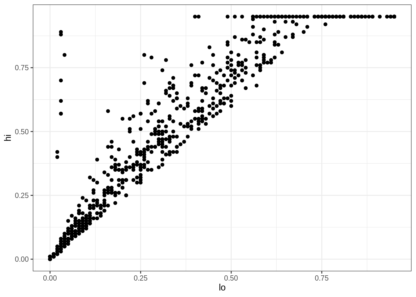
This plot immediately shows us that we have some outliers.
There are far more values with hi equal to 0.95 than it seems there ought to be, and there are eight points running up the left margin that seem troubling as well.
Let’s create a new tibble that doesn’t have these:
infant_hiv %>%
  drop_na() %>%
  filter(hi != 0.95) %>%
  filter(!((lo < 0.10) & (hi > 0.25))) %>%
  ggplot(mapping = aes(x = lo, y = hi, color = estimate)) +
  geom_point(alpha = 0.5) +
  xlim(0.0, 1.0) + ylim(0.0, 1.0) +
  theme_bw() +
  labs(x = 'Low estimate',
       y = 'High estimate',
       title = '% of infants born to women with HIV ... test themselves w/in two months of birth')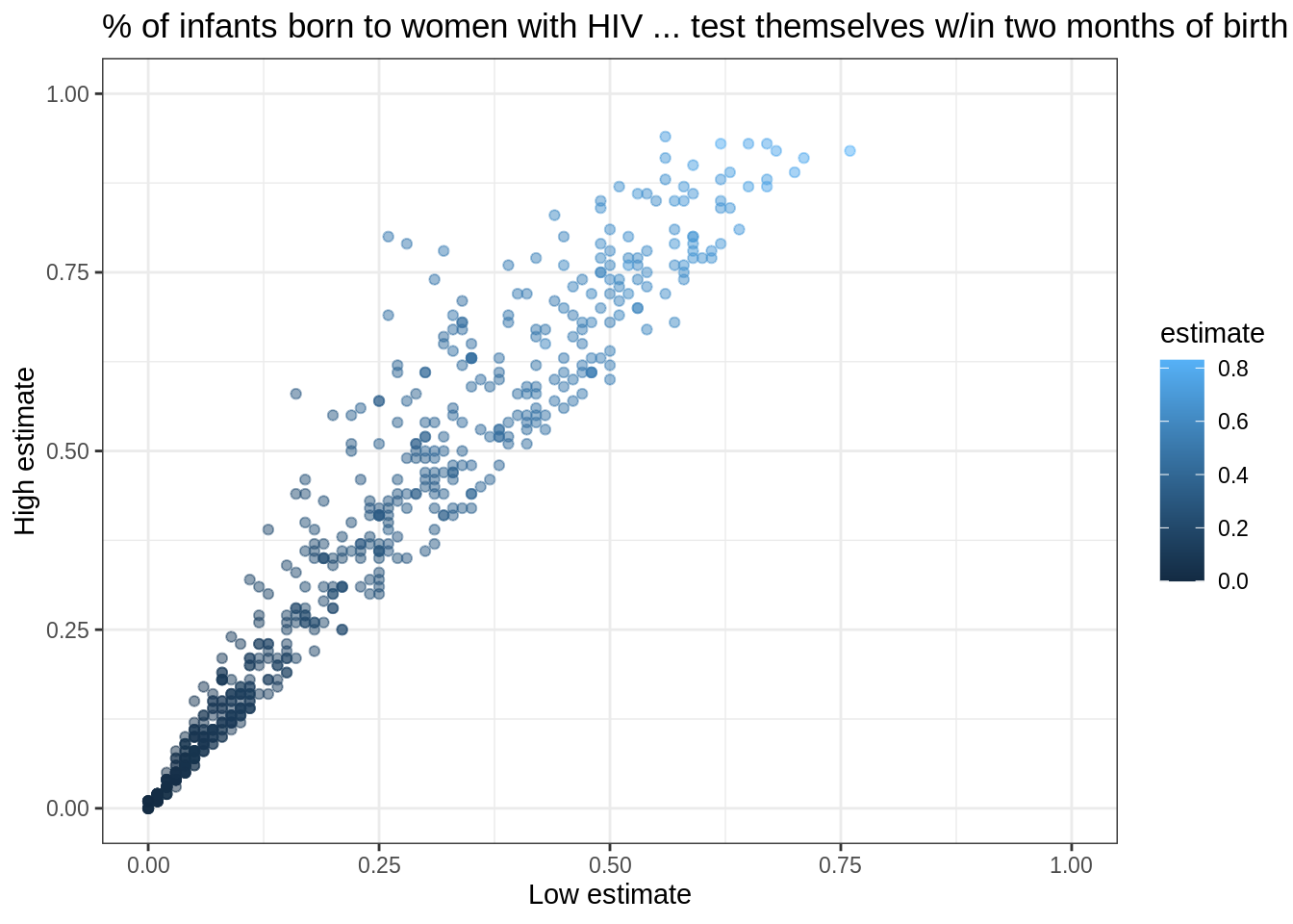
We can add the fitted curve by including another geometry called geom_smooth:
infant_hiv %>%
  drop_na() %>%
  filter(hi != 0.95) %>%
  filter(!((lo < 0.10) & (hi > 0.25))) %>%
  ggplot(mapping = aes(x = lo, y = hi)) +
  geom_point(mapping = aes(color = estimate), alpha = 0.5) +
  geom_smooth(method = lm, color = 'red') +
  xlim(0.0, 1.0) + ylim(0.0, 1.0) +
  theme_bw() +
  labs(x = 'Low estimate',
       y = 'High estimate',
       title = '% of infants born to women with HIV ... test themselves w/in two months of birth')
But wait: why is this complaining about missing values?
Some online searches lead to the discovery that geom_smooth adds virtual points to the data for plotting purposes, some of which lie outside the range of the actual data, and that setting xlim and ylim then truncates these.
(Remember, R is differently sane…)
The safe way to control the range of the data is to add a call to coord_cartesian, which effectively zooms in on a region of interest:
infant_hiv %>%
  drop_na() %>%
  filter(hi != 0.95) %>%
  filter(!((lo < 0.10) & (hi > 0.25))) %>%
  ggplot(mapping = aes(x = lo, y = hi)) +
  geom_point(mapping = aes(color = estimate), alpha = 0.5) +
  geom_smooth(method = lm, color = 'red') +
  coord_cartesian(xlim = c(0.0, 1.0), ylim = c(0.0, 1.0)) +
  theme_bw() +
  labs(x = 'Low estimate',
       y = 'High estimate',
       title = '% of infants born to women with HIV ... test themselves w/in two months of birth')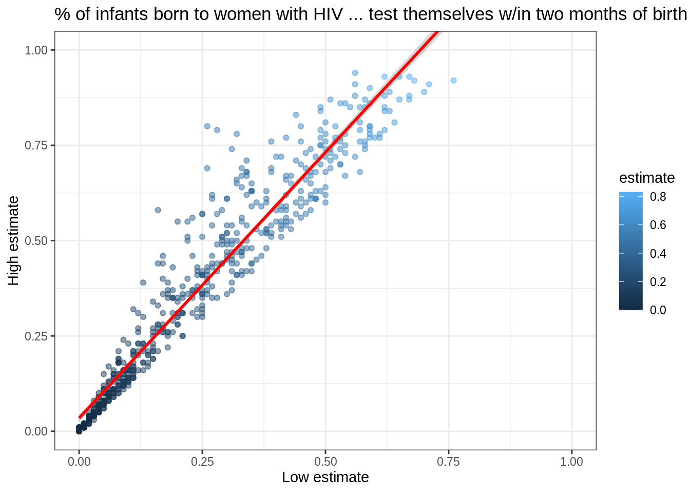
15.5.12 Do I need more practice with the tidyverse?
Absolutely!
First, accept your
participationassignment using GitHub classroomNavigate to the
cm101folder. Create a new subfolder inside here calleddata.In the
cm101_participation.Rmdfile, load theherepackage (recall it is used to construct paths without specifying user-specific paths).
- Download the person.csv file into the
datafolder you created.
- Next, use
here::hereto construct a path to a file andreadr::read_csvto read theperson.csvfile:
We don’t need to write out fully-qualified names—here and read_csv will do—but we will use them to make it easier to see what comes from where.
- Next, have a look at the tibble
person, which contains some basic information about a group of foolhardy scientists who ventured into the Antarctic in the 1920s and 1930s in search of things best left undisturbed:
## # A tibble: 5 x 3
##   person_id personal_name family_name
##   <chr>     <chr>         <chr>
## 1 dyer      William       Dyer
## 2 pb        Frank         Pabodie
## 3 lake      Anderson      Lake
## 4 roe       Valentina     Roerich
## 5 danforth Frank Danforth- How many rows and columns does this tibble contain?
## [1] 5## [1] 3(These names don’t have a package prefix because they are built in.)
- Let’s show that information in a slightly nicer way using
glueto insert values into a string andprintto display the result:
## person has 5 rows and 3 columns- Use the function
pasteto combine the elements of a vector to display several values.colnamesgives us the names of a tibble’s columns, andpaste’scollapseargument tells the function to use a single space to separate concatenated values:
## person columns are person_id personal_name family_name- Time for some data manipulation. Let’s get everyone’s family and personal names:
## # A tibble: 5 x 2
##   family_name personal_name
##   <chr>       <chr>
## 1 Dyer        William
## 2 Pabodie     Frank
## 3 Lake        Anderson
## 4 Roerich     Valentina
## 5 Danforth Frank- Then filter that list to keep only those that come in the first half of the alphabet:
## # A tibble: 3 x 2
##   family_name personal_name
##   <chr>       <chr>
## 1 Dyer        William
## 2 Lake        Anderson
## 3 Danforth Frank- It would be more consistent to rewrite this as:
## # A tibble: 3 x 2
##   family_name personal_name
##   <chr>       <chr>
## 1 Dyer        William
## 2 Lake        Anderson
## 3 Danforth Frank- Let’s add a column that records the lengths of family names:
## # A tibble: 5 x 4
## person_id personal_name family_name name_length
## <chr> <chr> <chr> <int>
## 1 dyer William Dyer 4
## 2 pb Frank Pabodie 7
## 3 lake Anderson Lake 4
## 4 roe Valentina Roerich 7
## 5 danforth Frank Danforth 8- Then arrange in descending order:
person %>%
dplyr::mutate(name_length = stringr::str_length(family_name)) %>%
dplyr::arrange(dplyr::desc(name_length))## # A tibble: 5 x 4
## person_id personal_name family_name name_length
## <chr> <chr> <chr> <int>
## 1 danforth Frank Danforth 8
## 2 pb Frank Pabodie 7
## 3 roe Valentina Roerich 7
## 4 dyer William Dyer 4
## 5 lake Anderson Lake 415.5.13 Key Points
install.packages('name')installs packages.library(name)(without quoting the name) loads a package.library(tidyverse)loads the entire collection of tidyverse libraries at once.read_csv(filename)reads CSV files that use the string ‘NA’ to represent missing values.read_csvinfers each column’s data types based on the first thousand values it reads.- A tibble is the tidyverse’s version of a data frame, which represents tabular data.
head(tibble)andtail(tibble)inspect the first and last few rows of a tibble.summary(tibble)displays a summary of a tibble’s structure and values.tibble$columnselects a column from a tibble, returning a vector as a result.tibble['column']selects a column from a tibble, returning a tibble as a result.tibble[,c]selects columncfrom a tibble, returning a tibble as a result.tibble[r,]selects rowrfrom a tibble, returning a tibble as a result.- Use ranges and logical vectors as indices to select multiple rows/columns or specific rows/columns from a tibble.
tibble[[c]]selects columncfrom a tibble, returning a vector as a result.min(...),mean(...),max(...), andstd(...)calculates the minimum, mean, maximum, and standard deviation of data.- These aggregate functions include
NAs in their calculations, and so will produceNAif the input data contains any. - Use
func(data, na.rm = TRUE)to removeNAs from data before calculations are done (but make sure this is statistically justified). filter(tibble, condition)selects rows from a tibble that pass a logical test on their values.arrange(tibble, column)orarrange(desc(column))arrange rows according to values in a column (the latter in descending order).select(tibble, column, column, ...)selects columns from a tibble.select(tibble, -column)selects out a column from a tibble.mutate(tibble, name = expression, name = expression, ...)adds new columns to a tibble using values from existing columns.group_by(tibble, column, column, ...)groups rows that have the same values in the specified columns.summarize(tibble, name = expression, name = expression)aggregates tibble values (by groups if the rows have been grouped).tibble %>% function(arguments)performs the same operation asfunction(tibble, arguments).- Use
%>%to create pipelines in which the left side of each%>%becomes the first argument of the next stage.